How to compare CNC machines by their lifetime carbon footprint

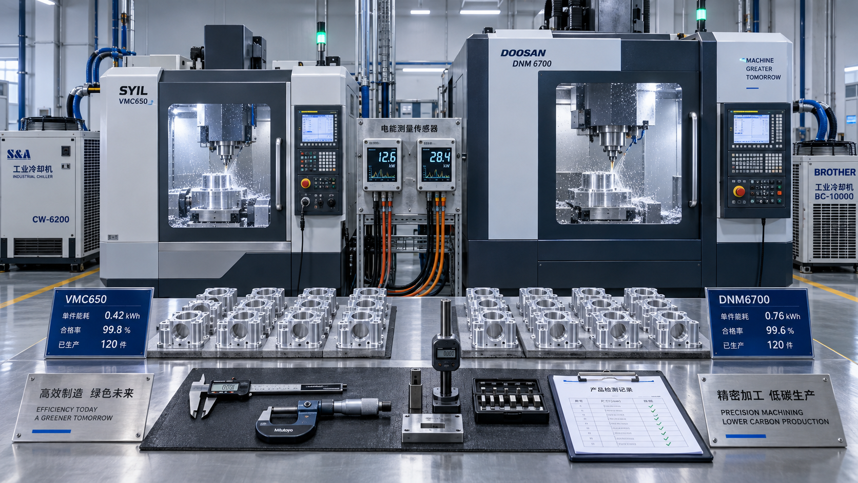
Compare CNC machines by the lifetime greenhouse gas emissions required to produce the same quantity of conforming parts. A machine with lower rated power can still have a larger footprint if it runs longer, rejects more components, or requires additional finishing operations. A heavier machine can justify its higher production footprint through lower operating emissions, provided the expected workload is sufficient to recover that difference.

Identifying low carbon footprint CNC machines therefore starts with a defined machining task, a realistic production schedule, and consistent accounting boundaries. Report both total lifetime emissions and emissions per accepted part. The first describes the overall carbon commitment; the second shows how effectively that commitment delivers useful production.

Fix the production requirement before comparing specifications

A fair comparison needs a common functional unit: a specified quantity of finished parts meeting the same requirements. Define the workpiece material and starting geometry, dimensional tolerances, surface finish, inspection criteria, and delivery rate. Include the operations needed to reach that condition, even when the candidate machines organize those operations differently.

For example, a multi-axis machining center might complete a component in one setup, while another configuration requires separate machining and finishing stages. Comparing only their individual cutting cycles would leave out handling, extra equipment, and the energy used between operations. Compare the complete production route through the agreed inspection point.

Keep the expected product mix visible. A machine optimized for continuous turning of similar steel shafts faces a different duty cycle from equipment producing small batches of complex aluminum housings. Tool changes, probing, setup, warm-up, and waiting time all affect energy per accepted part. A demonstration on a convenient sample part provides limited evidence for a substantially different workload.

The comparison must also satisfy capacity. If one machine cannot deliver the required annual output, include the additional equipment needed. Dividing each machine’s footprint by its theoretical maximum production conceals that practical difference.

Use a boundary that captures the equipment and its dependencies

Build the inventory around machine production, delivery and installation, operation, maintenance, and end-of-life treatment. Apply the same inclusions and exclusions to every candidate. Express greenhouse gas emissions as carbon dioxide equivalent, or CO₂e, using consistent calculation methods.

Shared services deserve particular attention. Compressed air, central coolant systems, extraction, and process cooling might draw power outside the machine’s electrical cabinet. Record their consumption separately and allocate it by a defensible measure, such as metered air demand or attributable cooling load. Avoid counting the same chiller in both cabinet measurements and a facility allocation.

Workpiece material requires an explicit accounting choice. Where identical material inputs are common to all options, their shared footprint can be held constant. Differences in blank size, scrap, and rejected parts must remain visible. A route that needs larger billets or loses more nearly finished components carries additional material emissions that electricity-only comparisons miss.

Measure energy across the actual production cycle

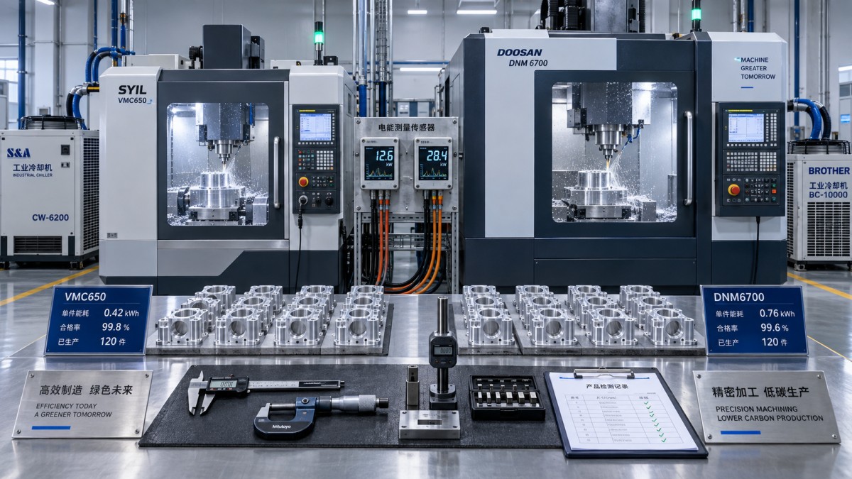
Rated spindle power describes capacity, not energy consumed per part. Measure electrical energy at a defined boundary while producing the agreed component, then relate the result to accepted output. Record the active machine configuration, cutting parameters, tool condition, coolant settings, and auxiliary equipment so that the measurement is reproducible.

A useful trial captures cold start and warm-up, setup, cutting, tool changes, probing, ready-state waiting, and shutdown. Extend the observation far enough to represent normal production. A short cutting test can miss the energy needed to maintain thermal stability or keep hydraulic and coolant systems running between batches.

Report measured kilowatt-hours alongside elapsed time and accepted part count. Separate cutting energy from the standing load where the data allows it. That distinction explains whether an improvement comes from more efficient machining, faster completion, or lower consumption while waiting.

A faster cycle can reduce energy per part even when instantaneous power rises, because pumps, controls, and cooling operate for less time. The result still needs confirmation at the required quality level. Aggressive cutting that accelerates tool wear, increases thermal drift, or creates extra rework shifts emissions elsewhere in the production route.

Energy-saving standby modes need a realistic restart test. If a shutdown requires lengthy warm-up before tight tolerances return, frequent switching can reduce the expected benefit. Measure the complete stop-and-restart sequence and confirm dimensional stability after restarting.

Account for rejected parts and tool consumption

Use accepted parts as the denominator, with consistent treatment of startup scrap, inspection failures, and rework. Energy consumed by a rejected component remains part of production emissions. Rework adds its own machine time and consumables, even when the component eventually passes inspection.

Cutting tools should be evaluated over a representative wear interval rather than with every trial starting on a fresh edge. Record tool life, replacement frequency, and the resulting quality distribution. A lower-energy cutting strategy loses some of its advantage if it consumes substantially more inserts or requires repeated corrective passes.

Turn measurements into a lifetime comparison

The basic calculation combines the emissions committed before operation with those expected during service and retirement:

Lifetime CO₂e = production + delivery and installation + operating electricity + consumables and maintenance + end-of-life treatment.

Apply recovery credits only where the selected accounting method allows them, and display them separately. Then divide the lifetime total by the expected number of conforming parts produced within that service scenario. If a machine processes several product families, allocate shared burdens using a consistent basis, such as occupied machine time, and disclose it.

Calculate operating electricity emissions using energy consumption and the electricity emission factor applicable to the production location. For a changing electricity supply, calculate successive periods separately. Do not apply a distant factory’s electricity factor to the intended installation site or assume that the current factor remains unchanged throughout service without testing that assumption.

Service life means productive life in the intended application. Mechanical durability alone does not establish how long a machine will remain useful. Control support, spare-part availability, repair options, and continued ability to meet tolerances affect the credible operating horizon. Include major rebuilds where they support the assumed life extension.

Utilization must come from the expected schedule. Allocate setup, warm-up, and idle energy across the output that schedule actually produces. Avoid combining maximum theoretical output with an energy estimate based on light use. If demand is fixed, evaluate both candidates against that demand over the same planning period, including replacements needed within it.

Find the carbon break-even point

Suppose one candidate has higher production and installation emissions but lower operating emissions per accepted part. Its extra initial burden is recovered only after sufficient output:

Break-even accepted parts = additional initial CO₂e ÷ operating CO₂e saved per accepted part.

This simplified expression assumes comparable service arrangements and reasonably stable emissions per part. Where maintenance events, changing electricity factors, or different yields materially affect the result, use a period-by-period calculation instead.

Compare the break-even output with credible demand before retirement. A machine that recovers its additional production footprint under continuous operation might never do so on intermittent prototype work. A cleaner electricity supply also reduces the carbon value of each kilowatt-hour saved, increasing the importance of machine production, repairs, and material losses.

Separate credible supplier evidence from unsupported claims

Supplier figures are useful only when their scope matches the comparison. Request the exact machine model and configuration, assessment boundary, calculation date, assumed lifetime, electricity factor, and production scenario behind any footprint claim. A figure for a basic machine does not describe a delivered cell with automation, extraction, and temperature-control equipment.

For production emissions, seek a documented material and component inventory or a model-specific life-cycle assessment. Identify which entries use measured supplier information and which rely on estimates. An independently reviewed assessment improves confidence in the method, but its assumptions still need to fit the intended application.

For operating claims, request the test program, workpiece specification, measured energy boundary, elapsed cycle time, quality results, and treatment of auxiliaries. A percentage reduction without a defined baseline cannot establish which candidate has the lower lifetime footprint.

Missing data should appear as an uncertainty range, rather than as zero emissions. Use the same estimation approach for comparable gaps across candidates. Keep evidence quality alongside the calculated result: a small apparent advantage supported by weak production data is less decisive than a larger advantage supported by representative measurements.

Test the assumptions that could reverse the choice

Build a base scenario from expected demand and the intended installation, then vary the assumptions with the greatest influence. Useful alternatives include lower utilization, a cleaner future electricity mix, shorter productive life, and a different reject rate. Keep each scenario physically consistent; fewer operating hours should also change output and the allocation of standing loads.

Examine which variable causes the ranking to reverse. If electricity dominates, measured energy and the site’s supply trajectory deserve priority. If utilization is low, machine production and service life carry greater weight. Where expensive blanks suffer significant rejection, process stability and material yield can determine the result.

Apply precision, surface finish, capacity, and reliability requirements as qualification gates before ranking carbon performance. Compare total cost of ownership alongside the carbon result using the same workload and maintenance assumptions. Electricity savings often support both objectives, while a carbon advantage dependent on uncertain tool life or extensive repairs requires closer examination.

The final comparison should retain the lifetime total, emissions per accepted part, evidence quality, and the conditions that change the ranking. When the apparent difference falls within the uncertainty of the inputs, targeted machining trials or better component data provide a stronger basis for selection than an extra decimal place.